Top CpGs

Adjusting for multiple testing

It is important to adjust p-values for multiple testing before performing any downstream analysis. The p.adjust method can be set to either:

fdr - less strict, often used for correlated measures like metabolites or
bonferroni - more strict, adjusts for all CpGs indepednently

limma_base <- limma_base %>% 
  mutate(padj = p.adjust(pval, method="fdr"))

Fetching top hits

After adjusting for multiple CpGs, top hits can be extracted and inspected.

top_cpgs <- limma_base %>% 
  filter(padj <= 0.05) %>% 
  arrange(padj)

print(paste0("There are ", 
             nrow(top_cpgs), " significant CpGs"))

## [1] "There are 106 significant CpGs"

print(paste0(nrow(top_cpgs %>% filter(beta<0)), 
             " of these are hypomethylated, and ", 
             nrow(top_cpgs %>% filter(beta>0)), 
             " are hypermethylated."))

## [1] "50 of these are hypomethylated, and 56 are hypermethylated."

Volcano plot

Significant CpGs can be visualized using a volcano plot. First limits for the plot are extracted.

if(nrow(top_cpgs) >= 1){
   sig_limit <- max(top_cpgs$p)
  } else {
  sig_limit <- 10E-07
  }

min <- as.numeric(min(
  abs(limma_base$beta),
  na.rm=TRUE))

max <- as.numeric(max(
  abs(limma_base$beta),
  na.rm=TRUE)) 

p_max <- as.numeric(-log10(min(limma_base$p, na.rm=TRUE))) + 2

Then the results can be visualized.

plot <- limma_base %>% 
  ggplot(aes(x = beta, y = -log10(p))) +
  geom_hline(yintercept = -log10(sig_limit),
             linetype = "dashed") +
  geom_point(color = ifelse(limma_base$p > sig_limit, 
                          "#BBBBBB","#4477AA")) +
  ylab(bquote(-log[10]~"p")) +
  xlab("Effect Size") +
  theme_bw()
print(plot)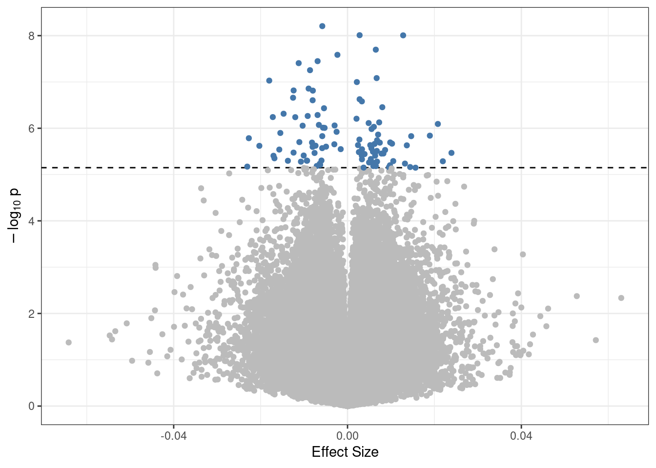

Enrichment analyses

Motivation

A simple list of CpGs gives little information about their relevance. Enrichment analyses can shine light on how best to interpret EWAS results and what may be driving the methylation signal.

Here we give an example for chromatin state enrichment, but a similar principle can be applied to investigate enrichment for trait associations using previous EWAS results or CpG islands, for example.

This is also only one type of follow-up analysis. Some other ideas include:

Performing bidirectional two-sample Mendelian randomization between DNAm at identified CpGs and the trait to infer causal directions.
Transcription factor binding site enrichment analysis using HOMER
Improving CpG-gene annotations with integrative analyses (e.g. using BIOS data) or genetic colocalization (e.g. using coloc)

Annotations

The Zhou lab GitHub page¹⁵ also provides Roadmap annotations for CpGs, on the basis of the original Roadmap reference epigenomes²⁸. These annotations can be imported to annotate measured CpGs to chromatin states.

First, we import the location annotations from before.

manifest_hg19 <- read_tsv(
  "./data/EPIC.hg19.manifest.tsv.gz")

## Rows: 865918 Columns: 57
## ── Column specification ───────────────────────────────────────────────────────────────────────────────────────────────────────────────────
## Delimiter: "\t"
## chr (21): CpG_chrm, probe_strand, probeID, channel, designType, nextBase, nextBaseRef, probeType, orientation, ProbeSeq_A, ProbeSeq_B, ...
## dbl (24): CpG_beg, CpG_end, address_A, address_B, probeCpGcnt, context35, probeBeg, probeEnd, beg_A, flag_A, mapQ_A, NM_A, beg_B, flag_...
## lgl (12): posMatch, MASK_mapping, MASK_typeINextBaseSwitch, MASK_rmsk15, MASK_sub40_copy, MASK_sub35_copy, MASK_sub30_copy, MASK_sub25_...
## 
## ℹ Use `spec()` to retrieve the full column specification for this data.
## ℹ Specify the column types or set `show_col_types = FALSE` to quiet this message.

anno <- manifest_hg19 %>% 
  dplyr::select(
    cpg = probeID,
    cpg_chr = CpG_chrm,
    cpg_start = CpG_beg,
    cpg_end = CpG_end,
    cpg_strand = probe_strand,
    gene_HGNC
  ) %>% 
  mutate(
    cpg_chr = substr(cpg_chr,4,5)
  )

anno <- anno %>% 
  dplyr::filter(cpg %in% limma_base$cpg)

Next, we import the chromatin state annotations. In this instance we use the PBMC (E062) reference epigenome, but there are reference epigenomes for many distinct cell types and tissues available²⁸. This is bound to the results data frame.

manifest_chrom <- read_tsv("./data/EPIC.hg19.REMC.chromHMM.tsv.gz")

## Rows: 865918 Columns: 131
## ── Column specification ───────────────────────────────────────────────────────────────────────────────────────────────────────────────────
## Delimiter: "\t"
## chr (129): CpG_chrm, probeID, E001, E002, E003, E004, E005, E006, E007, E008, E009, E010, E011, E012, E013, E014, E015, E016, E017, E01...
## dbl   (2): CpG_beg, CpG_end
## 
## ℹ Use `spec()` to retrieve the full column specification for this data.
## ℹ Specify the column types or set `show_col_types = FALSE` to quiet this message.

manifest_chrom <- manifest_chrom %>% 
  dplyr::select(cpg = probeID, E062)

anno <- left_join(anno, manifest_chrom, by="cpg")

limma_base <- left_join(limma_base, anno, by="cpg")

Running enrichment

Available states are stored as a vector.

states <- c("15_Quies", "14_ReprPCWk", "13_ReprPC", 
            "12_EnhBiv", "11_BivFlnk", "10_TssBiv", 
            "9_Het", "8_ZNF/Rpts", "7_Enh", 
            "6_EnhG", "5_TxWk", "4_Tx",  
            "3_TxFlnk", "2_TssAFlnk", "1_TssA")

Then, we can run the enrichment analysis using logistic regression.

for(i in states){
  res_road <- limma_base %>% 
    mutate(
      sig = ifelse(limma_base$cpg %in% top_cpgs$cpg, 1, 0),
      chrom = ifelse(grepl(i, E062), 1, 0)
    )
  
  x <- glm(chrom ~ sig, family=binomial, data=res_road)
  out <- c(coef(summary(x))[2,],
           exp(cbind(coef(x), confint.default(x)))[2,])
  names(out) <- c('logOR', 'SE', 'z', 'p', 'OR', 'low_CI', 'upp_CI')
  out <- as.data.frame(t(out))
  out$Trait = i
  out <- out %>% dplyr::select(Trait, OR, logOR, 
                               low_CI, upp_CI, z, p) 
  
  if(i == states[1]){
    res <- out
  } else {
    res <- rbind(res, out)
  }
}

P-values again need to be adjusted for multiple testing.

res$padj <- p.adjust(res$p, method='fdr')

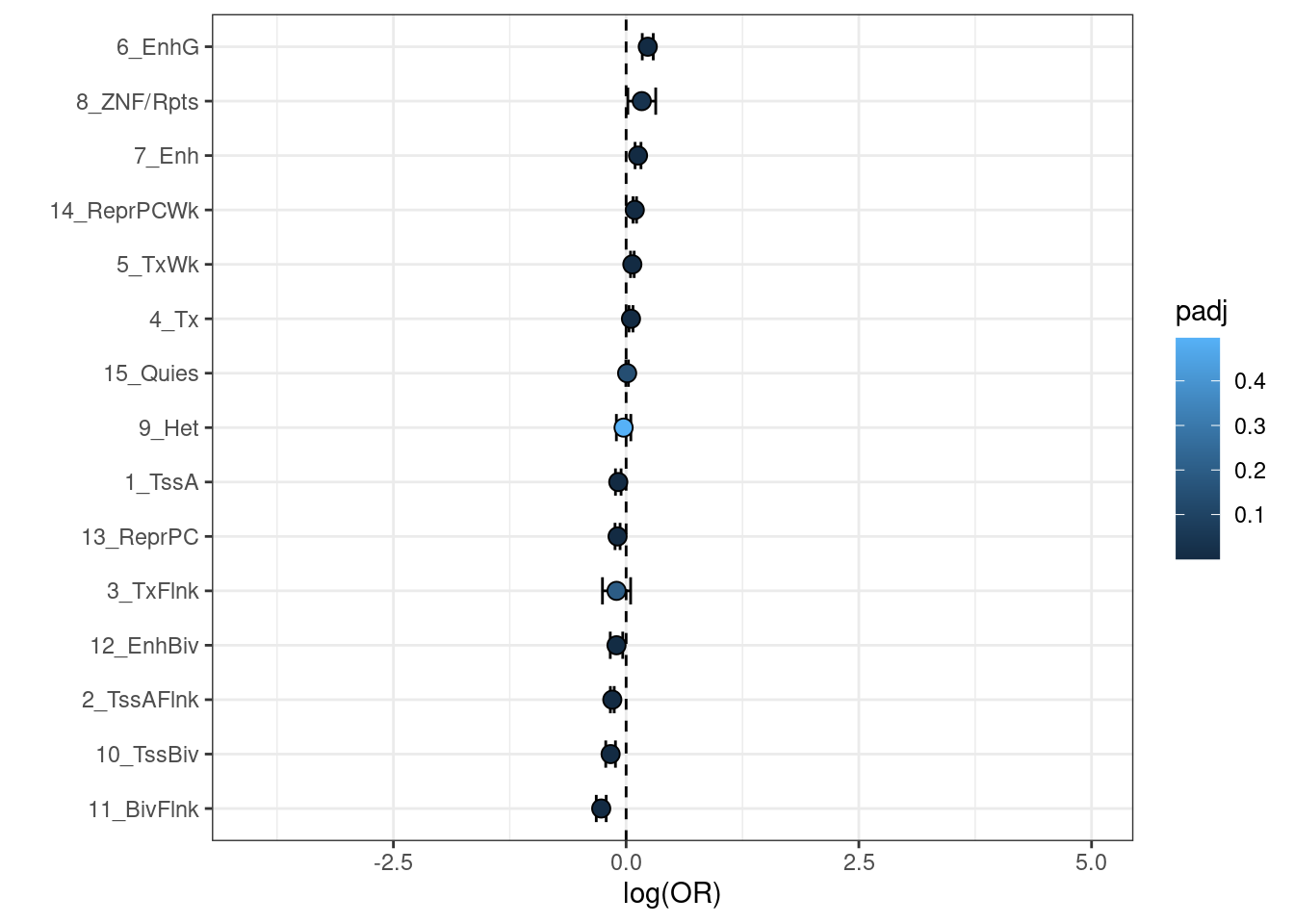
Visualization

These results can be visualized using a forest plot.

chrom <- res %>% 
  mutate(
    loglowCI = log(low_CI),
    loguppCI = log(upp_CI),
    padj = p.adjust(p, method='fdr')
  ) %>% 
  filter(OR < 200)

chrom %>% filter(padj < 0.05)

##        Trait       OR    logOR  low_CI   upp_CI        z            p         padj loglowCI loguppCI
## 1 8_ZNF/Rpts 23.79925 3.169654 8.75016 64.73074 6.208794 5.339283e-10 8.008925e-09 2.169072 4.170236

plot <- chrom %>% 
  filter(loglowCI > -4) %>% 
  ggplot(aes(x = logOR, 
             y = reorder(Trait,logOR),
             xmin = loglowCI,
             xmax = loguppCI)) +
  geom_vline(xintercept=0, linetype='dashed') +
  geom_errorbar(width=0.5,
                position=position_dodge(width=0.9)) +
  geom_point(aes(fill=padj),
             size=3,
             shape=21,
             position=position_dodge(width=0.9)) +
  xlab('log(OR)') + ylab('') + xlim(c(-4,5)) +
  theme_bw()
print(plot)