Covariates

Each column in the RGset colData should be considered as a potential covariate in EWAS models. Both technical and biological factors should be investigated as these may introduce batch effects or be clinically relevant. In order to assess this, you can visualize correlations with PCs as done previously in this workflow.

Any constant variables are removed from the heatmap, as they will not explain variance in the data.

plot_vars <- apply(targets, 2, function(x) sd(as.numeric(factor(x)), na.rm=T))

plot_vars <- names(plot_vars[!plot_vars %in% c(NA, 0)])
plot_vars

##  [1] "sample_ID"          "geo_accession"      "sex"                "age"                "log_total_pbb"      "pbb_153"           
##  [7] "pbb_77"             "pbb_101"            "pbb_180"            "supplementary_file" "plate"              "row"               
## [13] "Basename"           "CD4Tnv"             "Baso"               "CD4Tmem"            "Bmem"               "Bnv"               
## [19] "Treg"               "CD8Tmem"            "CD8Tnv"             "Eos"                "NK"                 "Neu"               
## [25] "Mono"

heatmap_df <- targets %>% 
  dplyr::select(any_of(plot_vars))

All variables are then converted to numeric and correlations between them and the PCs are calculated.

heatmap_df <- apply(heatmap_df, 2, function(x) as.numeric(factor(x)))

cxy <- round(cor(pca$x, scale(heatmap_df), use="pairwise.complete.obs"),2)

A heatmap can then be used to visualize these correlations and uncover measured variables that explain a large proportion of DNAm variance.

col_fun <- colorRamp2(c(-1, 0, 1), c("#000042", "white", "#800000"))

Heatmap(
  t(cxy),                              
  col = col_fun,  
  border = 'grey5',
  cluster_columns = FALSE,            
  show_row_dend = TRUE,             
  show_column_dend = FALSE,      
  name = "Value",                 
  row_names_gp = gpar(fontsize = 8), 
  column_names_gp = gpar(fontsize = 8), 
  cell_fun = function(j, i, x, y, width, height, fill) {
    grid.rect(x, y, width, height, 
              gp = gpar(col = "white", lwd = 1, fill = NA))
    grid.text(ifelse(abs(t(cxy)[i,j]) > 0.4,
                     sprintf("%.2f", round(t(cxy)[i, j], 2)),
                     ""), 
              x, y, gp = gpar(fontsize = 8, col = "white"))
  }
)

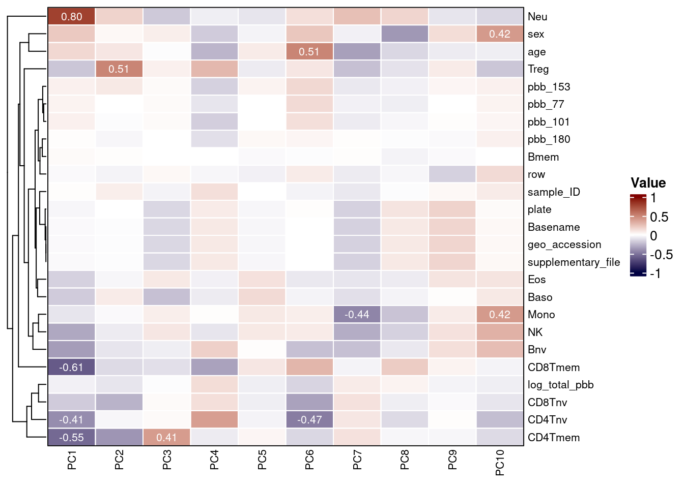
By examining the correlations in the data, we can build our model in a more informed manner. The second PC is highly correlated with sex and, as is usual in EWAS, we intend to include this as a confounder.

Some predicted cell counts appear of substantial importance and we advise also adjusting for these. Model specification should be informed by a combination of prior knowledge and inspection of patterns in the data.

SVA

Motivation

The sva package contains functions for removing batch effects and other unwanted variation in high-throughput experiments. Specifically, the sva package contains functions for the identifying and building surrogate variables for high-dimensional data sets. Surrogate variables are covariates constructed directly from high-dimensional data (like DNAm data) that can be used in subsequent analyses to adjust for unknown, unmodeled, or latent sources of noise.

The sva package can be used to remove artifacts in three ways:

identifying and estimating surrogate variables for unknown sources of variation in high-throughput experiments²³
directly removing known batch effects using ComBat²⁴, and
removing batch effects with known control probes²⁵

Removing batch effects and using surrogate variables in differential expression analysis have been shown to reduce dependence, stabilize error rate estimates, and improve reproducibility^23,26

Specification

The full model and null model are specified with and without the variable of interest respectively. In this case, we adjust for sex, age, plate, row, CD4Tnv, Baso, CD4Tmem, Bmem, Bnv, Treg, CD8Tmem, CD8Tnv, Eos, NK, and Mono. Neutrophils are excluded to avoid collinearity as all predicted cell counts sum to 1.

mod = model.matrix(~log_total_pbb + age + sex + plate + row + CD4Tnv + Baso + CD4Tmem + Bmem + Bnv + Treg + CD8Tmem + CD8Tnv + Eos + NK + Mono, data=targets)
mod0 = model.matrix(~age + sex + plate + row + CD4Tnv + Baso + CD4Tmem + Bmem + Bnv + Treg + CD8Tmem + CD8Tnv + Eos + NK + Mono,data=targets)

Imputation

Since SVA can only be run on complete data, we use methyLImp2²⁰ to create a complete matrix of beta values. The main function methyLImp2 can take a SummarizedExperiment or beta matrix as input, and requires the array type to be specified (as 450k or EPIC). By default it will overwrite your SummarizedExperiment object.

methData_imputed <- methyLImp2(
  input = methData, 
  type = "EPIC", 
  BPPARAM = SnowParam(exportglobals = FALSE),
  minibatch_frac = 0.5)

methData_imputed

## class: SummarizedExperiment 
## dim: 745368 57 
## metadata(0):
## assays(1): beta
## rownames(745368): cg09499020 cg16535257 ... cg08423507
##   cg24129471
## rowData names(8): cpg chr ... MASK_general probeType
## colnames(57): GSM3228563_200550980002_R02C01
##   GSM3228564_200550980002_R03C01 ...
##   GSM3228620_200590490021_R07C01
##   GSM3228621_200590490021_R08C01
## colData names(25): sample_ID geo_accession ... Neu Mono

Latent factor calculation

This can then be used to estimate the appropriate number of latent factors to calculate.

n.sv = num.sv(assay(methData_imputed),
              mod,
              method="leek")

The latent factors can then be calculated with the sva function:

svobj = sva(assay(methData_imputed),
            mod,
            mod0,
            n.sv=4)

## Number of significant surrogate variables is:  4 
## Iteration (out of 5 ):1  2  3  4  5

These can then be added to targets to include in the EWAS model.

sv_df <- as.data.frame(svobj$sv)
colnames(sv_df) <- c('SV1', 'SV2', 'SV3', 'SV4')
targets <- cbind(targets, sv_df)

EWAS

Packages

Limma²⁷ is a package with excellent documentation that can be useful for smaller samples, due to the optional empirical Bayes step. Other packages that may be of interest for running EWAS include [gee] and cate.

Formula

In order to run an EWAS a formula needs to be specified based on the above exploratory analyses and SVA.

formula <- ~log_total_pbb + age + sex + plate + row + CD4Tnv + Baso + CD4Tmem + Bmem + Bnv + Treg + CD8Tmem + CD8Tnv + Eos + NK + Mono + SV1 + SV2 + SV3 + SV4

You can then use this formula to create a design matrix.

design <- model.matrix(formula, 
                       data=targets)
head(design)

##                                (Intercept) log_total_pbb   age
## GSM3228563_200550980002_R02C01           1    -2.7535707 31.46
## GSM3228564_200550980002_R03C01           1    -0.3714986 46.72
## GSM3228565_200550980002_R04C01           1     0.1151128 46.36
## GSM3228566_200550980002_R05C01           1    -1.5478726 53.56
## GSM3228567_200550980002_R06C01           1    -0.9896682 56.36
## GSM3228568_200550980002_R07C01           1    -1.7620065 59.00
##                                sexMale plate200550980010
## GSM3228563_200550980002_R02C01       0                 0
## GSM3228564_200550980002_R03C01       1                 0
## GSM3228565_200550980002_R04C01       1                 0
## GSM3228566_200550980002_R05C01       0                 0
## GSM3228567_200550980002_R06C01       0                 0
## GSM3228568_200550980002_R07C01       0                 0
##                                plate200550980025
## GSM3228563_200550980002_R02C01                 0
## GSM3228564_200550980002_R03C01                 0
## GSM3228565_200550980002_R04C01                 0
## GSM3228566_200550980002_R05C01                 0
## GSM3228567_200550980002_R06C01                 0
## GSM3228568_200550980002_R07C01                 0
##                                plate200550980034
## GSM3228563_200550980002_R02C01                 0
## GSM3228564_200550980002_R03C01                 0
## GSM3228565_200550980002_R04C01                 0
## GSM3228566_200550980002_R05C01                 0
## GSM3228567_200550980002_R06C01                 0
## GSM3228568_200550980002_R07C01                 0
##                                plate200550980035
## GSM3228563_200550980002_R02C01                 0
## GSM3228564_200550980002_R03C01                 0
## GSM3228565_200550980002_R04C01                 0
## GSM3228566_200550980002_R05C01                 0
## GSM3228567_200550980002_R06C01                 0
## GSM3228568_200550980002_R07C01                 0
##                                plate200590490002
## GSM3228563_200550980002_R02C01                 0
## GSM3228564_200550980002_R03C01                 0
## GSM3228565_200550980002_R04C01                 0
## GSM3228566_200550980002_R05C01                 0
## GSM3228567_200550980002_R06C01                 0
## GSM3228568_200550980002_R07C01                 0
##                                plate200590490017
## GSM3228563_200550980002_R02C01                 0
## GSM3228564_200550980002_R03C01                 0
## GSM3228565_200550980002_R04C01                 0
## GSM3228566_200550980002_R05C01                 0
## GSM3228567_200550980002_R06C01                 0
## GSM3228568_200550980002_R07C01                 0
##                                plate200590490021 row     CD4Tnv
## GSM3228563_200550980002_R02C01                 0   2 0.11902209
## GSM3228564_200550980002_R03C01                 0   3 0.05644615
## GSM3228565_200550980002_R04C01                 0   4 0.06291340
## GSM3228566_200550980002_R05C01                 0   5 0.05244307
## GSM3228567_200550980002_R06C01                 0   6 0.02793638
## GSM3228568_200550980002_R07C01                 0   7 0.13030900
##                                       Baso    CD4Tmem       Bmem
## GSM3228563_200550980002_R02C01 0.000000000 0.06856902 0.04338180
## GSM3228564_200550980002_R03C01 0.003842171 0.06457686 0.03217819
## GSM3228565_200550980002_R04C01 0.000000000 0.09916235 0.03492393
## GSM3228566_200550980002_R05C01 0.000000000 0.08978173 0.02768882
## GSM3228567_200550980002_R06C01 0.000000000 0.10858777 0.04420792
## GSM3228568_200550980002_R07C01 0.004389993 0.10208036 0.02889159
##                                         Bnv       Treg    CD8Tmem
## GSM3228563_200550980002_R02C01 0.000000e+00 0.02987670 0.05170485
## GSM3228564_200550980002_R03C01 3.568496e-02 0.03253447 0.02588011
## GSM3228565_200550980002_R04C01 3.422224e-02 0.02091392 0.01348294
## GSM3228566_200550980002_R05C01 6.798882e-02 0.02574876 0.02891707
## GSM3228567_200550980002_R06C01 1.356557e-02 0.02396820 0.06586532
## GSM3228568_200550980002_R07C01 3.214358e-05 0.04655381 0.01622896
##                                     CD8Tnv         Eos         NK
## GSM3228563_200550980002_R02C01 0.064097832 0.001164834 0.03424776
## GSM3228564_200550980002_R03C01 0.000000000 0.012923973 0.06050254
## GSM3228565_200550980002_R04C01 0.000000000 0.002714143 0.02687347
## GSM3228566_200550980002_R05C01 0.005514883 0.013811095 0.11331037
## GSM3228567_200550980002_R06C01 0.000000000 0.007773618 0.02981967
## GSM3228568_200550980002_R07C01 0.003487802 0.000000000 0.03244102
##                                      Mono         SV1        SV2
## GSM3228563_200550980002_R02C01 0.07986611 -0.08479861 0.11245914
## GSM3228564_200550980002_R03C01 0.17395649 -0.10011645 0.04659800
## GSM3228565_200550980002_R04C01 0.09667953 -0.08706279 0.02731426
## GSM3228566_200550980002_R05C01 0.14498329 -0.07343356 0.17980275
## GSM3228567_200550980002_R06C01 0.07181471 -0.06994447 0.04691520
## GSM3228568_200550980002_R07C01 0.06782257 -0.08167816 0.04962268
##                                         SV3         SV4
## GSM3228563_200550980002_R02C01 -0.056605299  0.11744960
## GSM3228564_200550980002_R03C01  0.131833700 -0.05640994
## GSM3228565_200550980002_R04C01  0.124087644 -0.01504261
## GSM3228566_200550980002_R05C01  0.065412848  0.03247044
## GSM3228567_200550980002_R06C01  0.004589795  0.18848793
## GSM3228568_200550980002_R07C01  0.109370701 -0.34703374

Random effects

Random effects can be included using duplicateCorrelation and specifying the block argument. This is useful for paired experiments, not used in this example, but with example code shown here.

dupcor <- duplicateCorrelation(assay(methData),
                               design,
                               block = colData(methData)$ID)

Fitting models

Models are fit using lmFit.

fit <- lmFit(betas, design)

## Warning: Partial NA coefficients for 5 probe(s)

Models can also be fit for random effects using the dupcor object created above.

fit <- lmFit(betas, design,
             block = colData(methData)$ID,
             correlation = dupcor$consensus.correlation)

Extracting results

Results can then be extracted from the fit object, including the:

coefficients coef
standard errors se
t-statistics tstat
p-values pval, and
number of observations n

coef <- fit$coefficients[, 2]
se <- fit$stdev.unscaled[, 2] * fit$sigma
tstat <- coef / se
pval <- 2 * pt(-abs(tstat), fit$df.residual)
n <- ncol(design) + fit$df.residual

`bacon`

Motivation

We developed a package called bacon¹¹ to estimate and correct for bias and inflation of test statistics in EWAS. This maximizes power while properly controlling the false positive rate, by estimating the empirical null distribution using Bayesian statistics. The utility of the tool was illustrated through the application of meta-analysis by performing epigenome- and transcriptome-wide association studies (EWASs/TWAS) on age and smoking which highlighted an overlap in differential methylation and expression of associated genes.

Adjusting for bias and inflation

We advise using bacon to estimate inflation and bias often observed in EWAS. This object can then be printed to report the estimated bias and inflation.

bc <- bacon(teststatistics = tstat,
            effectsizes = coef,
            standarderrors = se,
            verbose = TRUE)

## Use multinomial weighted sampling...

## threshold = -5.3985
## Starting values:
## p0 = 1.0000, p1 = 0.0000, p2 = 0.0000
## mu0 = 0.0040, mu1 = 5.5135, mu2 = -5.5055
## sigma0 = 1.0206, sigma1 = 1.0206, sigma2 = 1.0206

bc

## Bacon-object containing 1 set(s) of 745368 test-statistics.
## ...estimated bias: 0.0047.
## ...estimated inflation: 1.
## 
## Empirical null estimates are based on 5000 iterations with a burnin-period of 2000.

P-values and t-statistics can then be adjusted

pval <- bacon::pval(bc)
tstat <- bacon::tstat(bc)

Plots

Bacon also provides some visualizations of its performance, which can come in handy.

print(plot(bc, type="hist"))

## `stat_bin()` using `bins = 30`. Pick better value with `binwidth`.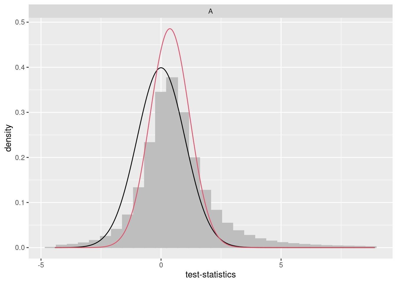

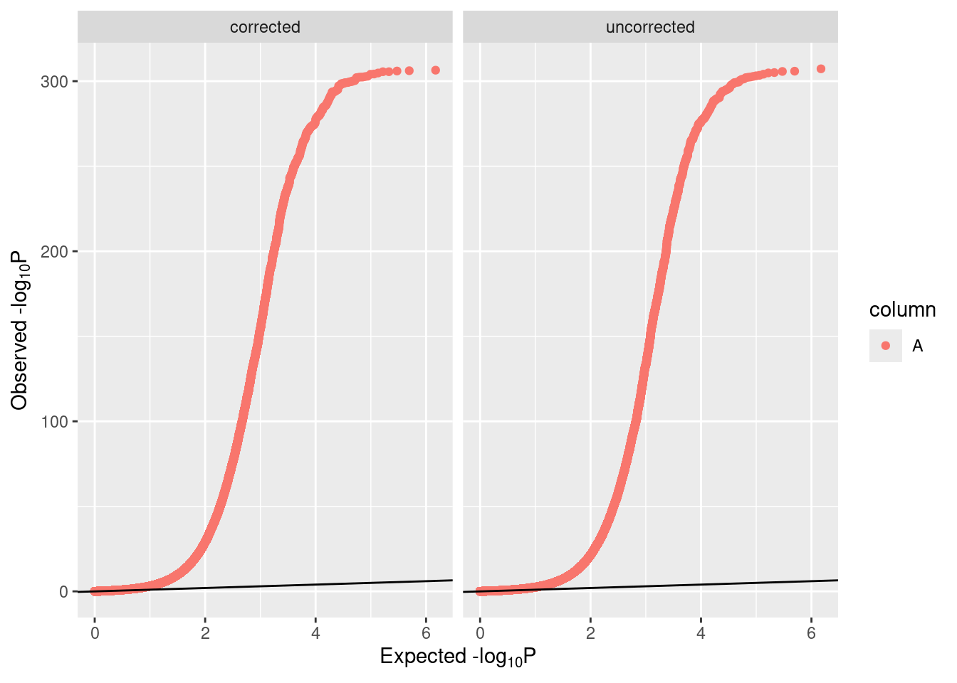
print(plot(bc, type="qq"))

Additionally, rerunning bacon can provide an estimate of any residual bias or inflation.

bc <- bacon::bacon(teststatistics = tstat,
                   effectsizes = coef,
                   standarderrors = se,
                   verbose = TRUE)

## Use multinomial weighted sampling...

## threshold = -5.3985
## Starting values:
## p0 = 1.0000, p1 = 0.0000, p2 = 0.0000
## mu0 = -0.0007, mu1 = 5.4171, mu2 = -5.4185
## sigma0 = 1.0036, sigma1 = 1.0036, sigma2 = 1.0036

bc

## Bacon-object containing 1 set(s) of 745368 test-statistics.
## ...estimated bias: 0.00018.
## ...estimated inflation: 1.
## 
## Empirical null estimates are based on 5000 iterations with a burnin-period of 2000.

Saving results

Bacon-adjusted results can then be saved, for use in downstream analysis.

limma_base <- data.frame(cpg = rownames(fit$coefficients), 
                         beta = coef, SE = se, 
                         p = pval, 
                         t = tstat, N = n)