---

Normalization

Motivation

Our workflow outline the use of functional normalization¹⁶, which exploits internal control probes designed to detect technical variations without assaying biological differences, and dasen as implemented by wateRmelon³⁰. Both are adjusted and updated to use the interpolatedXY method³¹.

Functional normalization has been shown to perform favourably when compared to other approaches¹⁷. Using the internal control probes avoids the problems associated with global normalization methods, where biological variation can be mistaken for a technical effect and removed. This is especially important in studies where groups are expected to have differential methylation signatures, such as multiple tissue studies¹⁸.

Conversations on the best approaches for normalization in DNAm data pipelines are ongoing¹⁹.

---

Principal Components

The default of selecting only two principal components is often too low for this type of data. Often you will see a drop-off in proportion of variance explained after a certain number of principal components, and this can indicate an efficient selection.

var_explained %>% ggplot(aes(x=PC, y=var_explained)) +
  geom_line() +
  geom_point(color='grey5', fill='#6DACBC', shape=21, size=3) + 
  scale_x_continuous(breaks=1:ncol(pca$x)) +
  xlab("Principal Component") + 
  ylab("Proportion of variance explained") +
  theme_bw()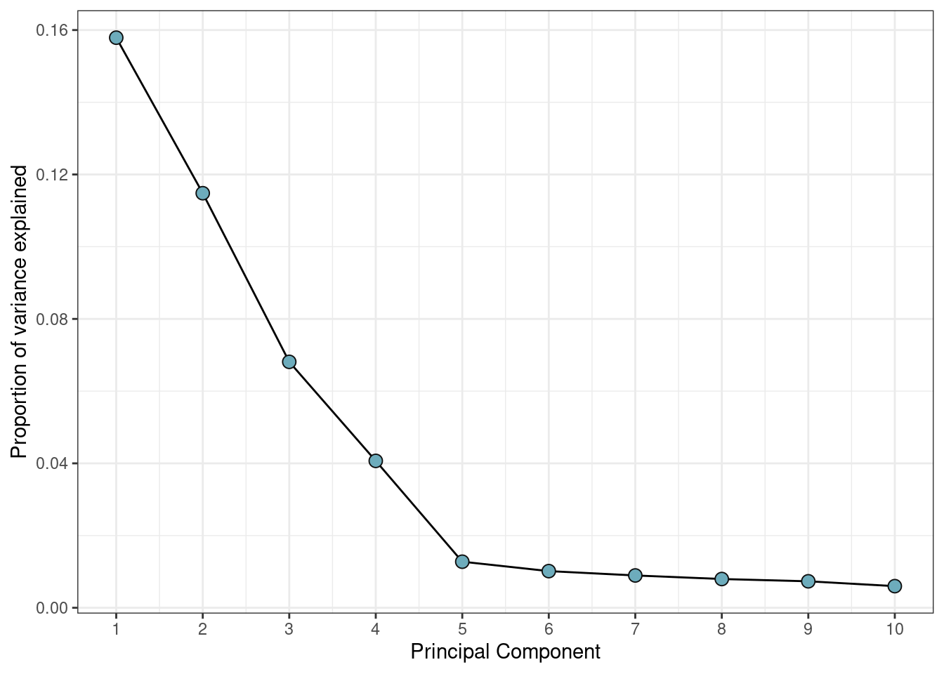

---

Running Normalization

In order to run normalization the annotation of the RGset must be updated for EPIC arrays.

RGset@annotation <- c(array = "IlluminaHumanMethylationEPIC", annotation = "ilm10b4.hg19")

We use the adjustedFunnorm function from wateRmelon, which uses the interpolated XY method³¹. By default, functional normalization returns normalized copy number data making the returned GenomicRatioSet twice the size necessary when only beta-values or M-values are required. Therefore, we set keepCN to FALSE.

GRset <- adjustedFunnorm(
  rgSet = RGset,
  nPCs = 4,
  sex = ifelse(targets$sex == "Female", 0, 1),
  keepCN = F,
  verbose = T
)

## [adjustedFunnorm] Background and dye bias correction with noob

## [adjustedFunnorm] Mapping to genome

## [adjustedFunnorm] Quantile extraction

## [adjustedFunnorm] Normalization

GRset

## class: GenomicRatioSet 
## dim: 865859 496 
## metadata(0):
## assays(1): Beta
## rownames(865859): cg14817997 cg26928153 ... cg07587934 cg16855331
## rowData names(0):
## colnames(496): GSM3228585_200550980034_R01C01
##   GSM3228586_200550980034_R02C01 ... GSM3229237_200598350015_R06C01
##   GSM3229239_200598350080_R03C01
## colData names(25): sample_ID geo_accession ... Neu Mono
## Annotation
##   array: IlluminaHumanMethylationEPIC
##   annotation: ilm10b4.hg19
## Preprocessing
##   Method: NA
##   minfi version: NA
##   Manifest version: NA

It is also possible to use adjustedDasen to apply dasen normalization to normalize autosomal CpGs and infer the sex chromosome linked CpGs by linear interpolation on corrected autosomal CpGs. Instead of outputting a GRset, this function outputs the normalized beta values. Therefore, using this normalization removes the need for the DNAmArray reduce function in the next steps.

betas <- adjustedDasen(mns = methylated(RGset),
                       uns = unmethylated(RGset),
                       onetwo = fData(RGset)[,fot(RGset)], 
                       chr = fData(RGset)$CHR)

---